A Join A Day – The Hash Join

Introduction

This is the twenty-third post in my A Join A Day series about SQL Server Joins. Make sure to let me know how I am doing or ask your burning join related questions by leaving a comment below.

The Hash Join algorithm is a good choice, if the tables are large and there is no usable index. Like the Sort Merge Join algorithm, it is a two-step process. The first step is to create an in-memory hash index on the left side input. This step is called the build phase. The second step is to go through the right side input one row at a time and find the matches using the index created in step one. This step is called the probe phase.

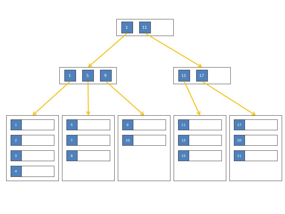
The Hash Join Algorithm

Usually a hash join execution plan contains only one icon for the entire process of building the hash table and using it to do the actual join. However, in SQL Server 2012 you might in some special cases see a separate icon for the build phase:

The first step in the Hash Join algorithm is always to create a hash index (or hash table) for the left side input. A hash index gets created by distributing the rows into several buckets. Each bucket is a memory area with a distinct address that can hold a group of rows. All the columns from the left side that are needed later in the query are included and stored in those buckets. Therefore the memory requirement is proportional to the size of the left side input.

The address of the bucket to store a given row is calculated using a hash function over the columns that are part of the join condition. A hash function is a deterministic function that transforms an input of one or more columns into a single number. Every time the same input is used, the same number will result. However, it is possible and even likely that two different inputs will yield the same number.

In an equi-join all columns of the join condition are included in the calculation of the hash value. In a nonequi-join condition only the columns that use an equality comparison are included in that calculation. That means that the Hash Join algorithm does not work if there is not at least one equality column included in the join condition.

Once all rows of the first input are distributed amongst the buckets, SQL Server loops through the rows of the second input one at a time. For each row it takes the equality columns of the join condition and calculates the hash value using the same hash function that was used in the creation of the hash table. Any matching row must be in the bucket with the same address. However, because the hash function might result in the same value for differing inputs, we can't tell at this point which of the rows in that bucket – if any – join to the current row. The only way to find out is to loop through all of them basically executing a nested loop. So the fewer rows there are in each bucket, the more efficient this algorithm works. A good hash function causes the input data to be evenly distributed amongst all available buckets.

The Hash Join algorithm is able to handle any of the logical join types. If the join is a Left Outer Join, a Full Outer Join or a Left Anti Semi Join, a marker is added to each row in the hash index to keep track of rows that had a match. At the end of the join process a single scan of the hash index will return all unmatched rows.

In the beginning of this article I stated that the hash index is an in-memory construct. So what happens if there is not enough memory? In that case SQL Server uses a complicated algorithm paging sections of the hash table in and out of memory. See http://msdn.microsoft.com/en-us/library/aa178403(v=sql.80).aspx for a little more detail on this. This paging of data between memory and disk can be quite a drain on the available resources. The hash table components that need to be moved out of memory are stored in tempdb. This process is called "spilling".

Let's look at an example. We are going to reuse the same two tables we have used for the Nested Loop Join and the Merge Join. Here is what they look like again:

Let's run the following query, this time with a hash join hint:

It will produce these statistics:

Again, like with the Merge Join algorithm, both tables get scanned completely once each. There is also again a Worktable mentioned that was not read from. The worktable has been created to provide a place to store the pieces of the hash index that had to be paged out due to memory constraints. It has 0 logical reads in this example which means its use was not necessary.

Sort Hash Join Strengths and Weaknesses

Because the Hash Join like the Sort Merge Join has a setup phase, there is a setup cost involved. This setup cost is due to the creation of the in-memory hash table. While that process is not complicated, it will take time and a lot of memory. Below are the characteristics of the Hash Join algorithm.

• + All logical join types can be handled.
• - There is a substantial setup cost.
• - It does require a sizable amount of memory, big enough to fit the entire left side input. (Spilling to tempdb is possible)
• - During the entire time it takes to create the hash index, no row will be returned.
• - At least one column in the join condition needs to use an equality comparison.

All over all this is the most resource intensive join algorithm because of the expensive build phase. However, once the hash table is build, this join algorithm can be quite fast. For large tables with no usable index, the time savings during the probe phase will more than outweigh the additional cost of the build phase. Keep in mind however that because of the large memory requirements, only very few of these can run at the same time.

Summary

A Join A Day

This post is part of my December 2012 "A Join A Day" blog post series. You can find the table of contents with all posts published so far in the introductory post: A Join A Day – Introduction. Check back there frequently throughout the month.