A Join A Day – Predicate, Probe & Residual
Introduction
This is the twenty-fourth post in my A Join A Day series about SQL Server Joins. Make sure to let me know how I am doing or ask your burning join related questions by leaving a comment below.
The different join algorithms have different ways of identifying rows that need to be checked for a possible match. We did look at that in detail over the last three days. Today we are going to look at the details of the actual matching process.
The Probe
To start out let's take a look at this simple Hash Join query:
FROM Sales.SalesOrderDetail AS sod
INNER HASH JOIN Sales.SalesOrderHeader AS soh
ON sod.SalesOrderID = soh.SalesOrderID;
[/sql]
It produces this execution plan:

If you look at the properties for the Hash Join operator you see a "Hash Key Build" and a "Hash Key Probe". The build hash key is used when the hash index is created. The probe hash key is then used to find the bucket with match candidates in that index for each row from the second input. Each contains the list of columns from one side that use an equality comparison in the join condition. So what happens when there is an inequality column?
The Residual
To find out let's add an inequality column to our query:
FROM Sales.SalesOrderDetail AS sod
INNER HASH JOIN Sales.SalesOrderHeader AS soh
ON sod.SalesOrderID = soh.SalesOrderID
AND sod.ModifiedDate != soh.ModifiedDate;
[/sql]
Now the query has one equality and one inequality column. Remember, that only equality columns can be used for the hash key. So something else needs to happen with the inequality column. The execution plan looks pretty much identical at first:

However that is now one additional property in the properties list of the Hash Join operator. It is the "Probe Residual" and this is its value (with added linebreaks):
[AdventureWorks2008R2].[Sales].[SalesOrderHeader].[SalesOrderID] as [soh].[SalesOrderID] AND
[AdventureWorks2008R2].[Sales].[SalesOrderDetail].[ModifiedDate] as [sod].[ModifiedDate] <>
[AdventureWorks2008R2].[Sales].[SalesOrderHeader].[ModifiedDate] as [soh].[ModifiedDate] [/sourcecode]
The Probe Residual property can only be found if there are columns in the join condition that could not be part of the hash key. However, the probe only identifies the correct bucket. To identify all matching rows in there SQL Server has to compare each of them with the current one. This comparison is using the value of the Probe Residual as condition. The Probe residual therefore matches the join condition of the query. This is even the case if there are only equality columns in the condition. In that case the residual is just not spelled out for us.
Where (join columns)
Let's look at the same query with a merge join hint:
FROM Sales.SalesOrderDetail AS sod
INNER MERGE JOIN Sales.SalesOrderHeader AS soh
ON sod.SalesOrderID = soh.SalesOrderID
AND sod.ModifiedDate != soh.ModifiedDate
[/sql]
The execution plan now contains a Merge Join Operator. Its properties look very similar to the ones of the Hash Join operator:

The main difference is that the join condition now is not represented by a set of keys, but by a "Where (join columns)" section. This section also contains only equality columns. The complete join condition can be found in the "Residual" property. The value of the Residual property for above query looks like this:
[AdventureWorks2008R2].[Sales].[SalesOrderHeader].[SalesOrderID] as [soh].[SalesOrderID] AND
[AdventureWorks2008R2].[Sales].[SalesOrderDetail].[ModifiedDate] as [sod].[ModifiedDate] <>
[AdventureWorks2008R2].[Sales].[SalesOrderHeader].[ModifiedDate] as [soh].[ModifiedDate] [/sourcecode]
Other than with Hash Join operators, this property is present on equi-merge-joins:

Unsurprising its value is this:
[AdventureWorks2008R2].[Sales].[SalesOrderDetail].[SalesOrderID] as [sod].[SalesOrderID] [/sourcecode]
This makes sense, as the "join columns" really are only used to sort the two inputs. The final comparison using the residual is what decides if the two rows are a match or not.
Out of the Loop
After looking at the Hash Join and Merge Join operators there is one more left to dissect. It is the Loop Join operator, and with it things are different. But let's look at an example first:

This is the same query we have used before, this time with a loop join hint. The properties of the Loop Join operator contain the join condition — nowhere?! There is no indication on this operator anywhere that would tell us what the join condition is. But if you remember the Cross Join article, SQL Server does complain if there is no condition given. That means, as there is no warning in this plan that it did not miss this one's condition. So what happened?
The Predicate
The data access operator for the Sales.SalesOrderHeader table, which makes the right side input to our join, is a Seek operator. For a seek you need a value to seek for. That search value in an index seek is called "Seek Predicate" and you can find it in the properties of the Index Seek operator:

It contains this value:
[/sourcecode]
This is a little cumbersome to read but it says that the SalesOrderId column in the Sales.SalesOrderHeader need to match that of the SalesOrderId column in the Sales.SalesOrderDetail table. This matches the equality part of our join condition.
There is a second property on the Index Seek operator, the "Predicate" property. It contains this value:
[AdventureWorks2008R2].[Sales].[SalesOrderHeader].[ModifiedDate] as [soh].[ModifiedDate] [/sourcecode]
This is just the inequality part of the join condition. So within the Index Seek operator SQL Server directly accesses only rows that are a match in one part of the join condition. Those rows get passed through an additional filter within the same operator that takes care of the second half of the join condition. So, all rows that reach the Nested Loops Join operator are known to be a match already. Therefore that operator does not need to know about the join condition anymore and can just combine all rows coming back from the index seek with the current row from the Sales.SalesOrderHeader table.
The columns included in the Seek Predicate are not necessarily all of the equality columns. Instead it is the largest index key prefix that is completely part of the equality section of the index. So if the join condition would be t1.a = t2.a AND t1.b = t2.b and t2 had an index on the columns a, c the Seek Predicate would contain just column a.
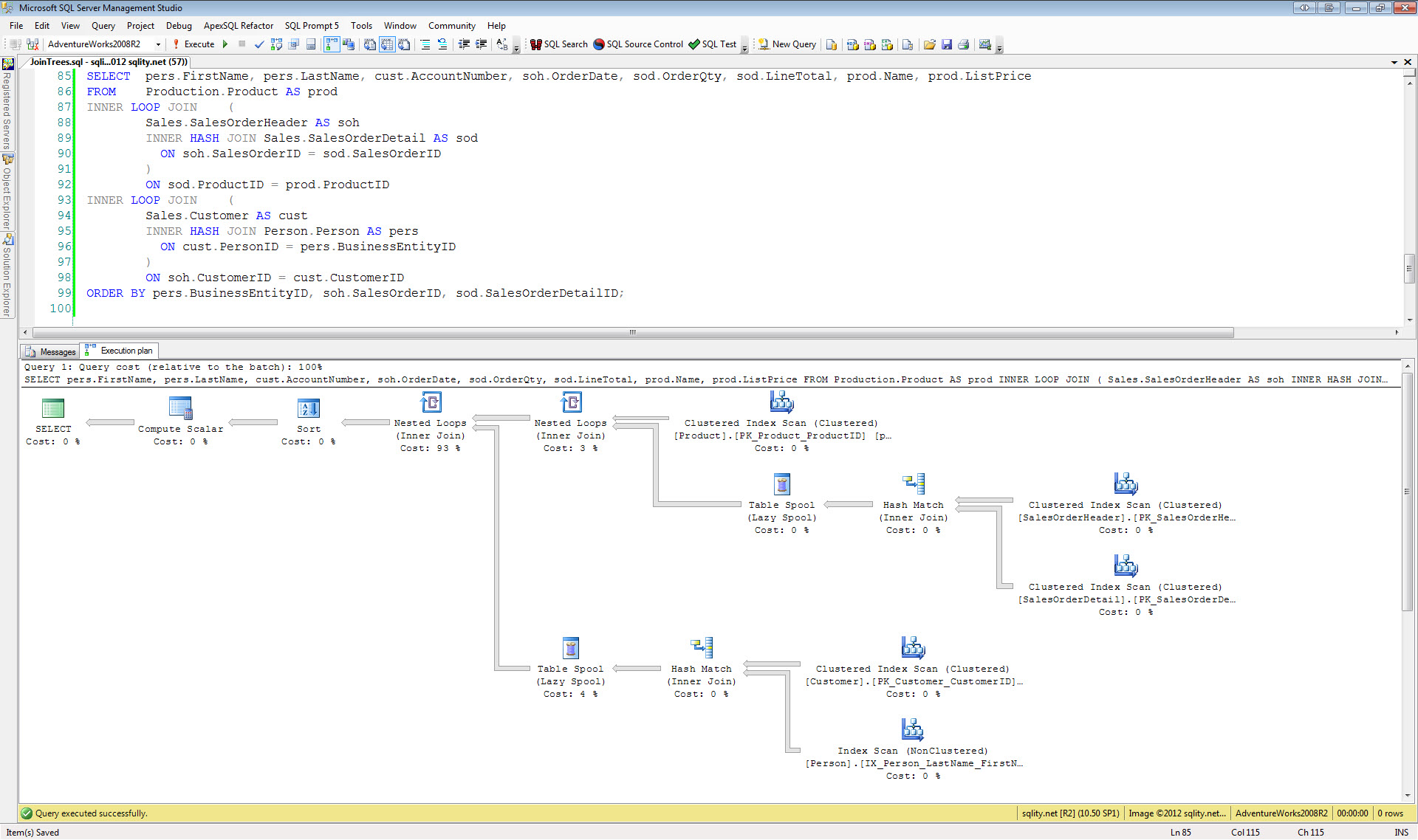
The previous example showed a loop join that was able to make use of an index on the right side table. Let's see what happens if that is not possible. For the purpose of this exercise let's assume we are looking for all Sales.SalesOrderDetail records to a given Sales.SalesOrderHeader row that happened on the same day but are associated with a different order:
SELECT soh.AccountNumber, sod.OrderQty, sod.UnitPrice
FROM Sales.SalesOrderDetail AS sod
INNER LOOP JOIN Sales.SalesOrderHeader AS soh
ON sod.SalesOrderID != soh.SalesOrderID
AND sod.ModifiedDate = soh.ModifiedDate;
SET ROWCOUNT 0;
[/sql]
The two SET ROWCOUNT statement restrict the number of rows coming back from the query in between to 50 rows. I did not want to wait for this query to finish without that restriction.
The execution plan for this query looks the same as the one of the previous query with the exception of the arrow thickness:

The properties for the Loop Join operator contain one called "Predicate". It contains the following value:
[AdventureWorks2008R2].[Sales].[SalesOrderHeader].[ModifiedDate] as [soh].[ModifiedDate] AND
[AdventureWorks2008R2].[Sales].[SalesOrderDetail].[SalesOrderID] as [sod].[SalesOrderID] <>
[AdventureWorks2008R2].[Sales].[SalesOrderHeader].[SalesOrderID] as [soh].[SalesOrderID] [/sourcecode]
This contains the entire join condition with both the equality part and the inequality part. So, all rows from the second input get passed into the join operator in this case to build the complete Cartesian product. The join operator then identifies the matches using the Predicate value.
This showed the two extreme examples of Loop Join implementations in SQL Server. Depending on the query anything in between could happen too. Sometimes you even see an additional Filter operator in between the table access operator and the right side input of the Loop Join operator.
Summary
This article showed the different places where the join condition can be found in a join execution plan. We covered Predicates, Probes and Residuals which are used to identify the matching rows in different places of the plan. Which ones are actually part of a given plan is depending on the join operator used.
A Join A Day
This post is part of my December 2012 "A Join A Day" blog post series. You can find the table of contents with all posts published so far in the introductory post: A Join A Day – Introduction. Check back there frequently throughout the month.
Newsletter Sign Up

We know how to make a database not slow. We’ll help you do the same.
From the sqlity.net blog
-
How to identify the SQL Server Service Account in T-SQL

-
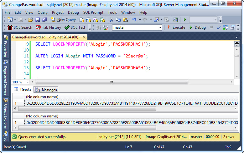
How to Change a SQL Login’s Password
-
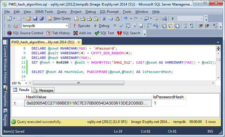
Hash Algorithms – How does SQL Server store Passwords?
-
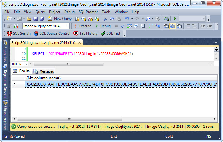
How to Re-Create a Login with only a Hashed Password
-
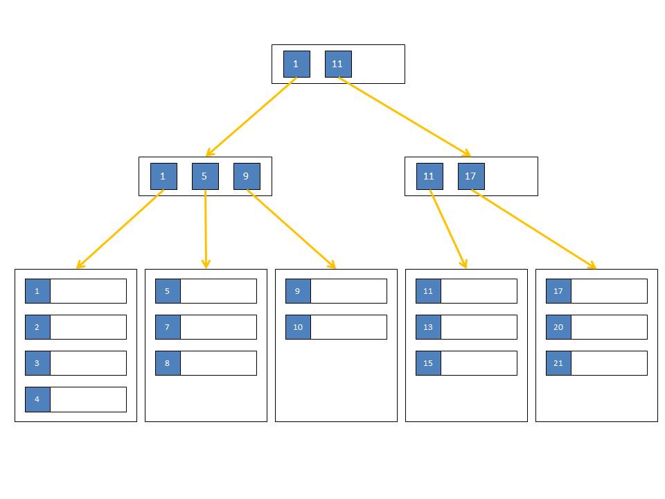
B+Trees – How SQL Server Indexes are Stored on Disk
-
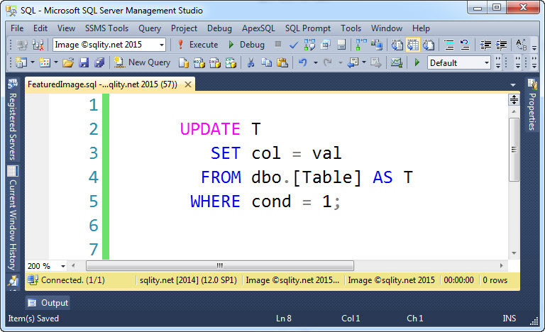
The Hidden SQL Server Gem: UPDATE from SELECT
-
A Join A Day – Nested Joins
-
Determine the Uptime of a SQL Server Instance

-
A Join A Day – The Left Anti Semi Join
-
Log Reuse Waits Explained: LOG_BACKUP